Changing Summary Calculations
When
creating your pivot table report, Excel will, by default, summarize
your data by either counting or summing the items. Instead of Sum or
Count, you might want to choose functions, such as Average, Min, Max,
and so on. You can easily change the summary calculation for any given
field by following these steps.
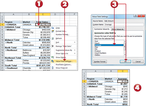
1. Right-click any value within the target field.
2. Select Value Field Settings.
3.
The Value Field Settings dialog box appears. Choose the type of
calculation you want to use from the list of calculations, then click OK to confirm.
4. Note that the pivot table now shows your chosen calculation.
Note: How Excel Chooses Sum or Count
When
you click on a numeric field in the PivotTable Field List, Excel
automatically places that field in the Values area. However, Excel
doesn’t necessarily apply a Sum to that field. If all the cells in a
column contain numeric data, Excel chooses a Sum calculation by default.
However, if just one cell in that same column is either blank or
contains text, Excel chooses the Count calculation. |
Showing and Hiding Data Items
A
pivot table summarizes and displays all the records in your source data
table. There may, however, be situations when you want to inhibit
certain data items from being included in your pivot table summary. In
these situations, you can choose to hide a data item. In terms of pivot
tables, hiding doesn’t just mean preventing the data item from being
shown on the report, hiding a data item also prevents it from being
factored into the summary calculations. For example, you can hide the
Canada market to see only sales for U.S. markets.
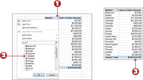
1. Click on the drop-down for the field you are filtering—in this case, the Market field.
2. Remove the check from the data item you want hidden. Here, Canada is being removed so that only U.S. sales are calculated.
3.
After the filter has been applied, you’ll note that not only is the
Canada market hidden, but the grand total has recalculated to show the
total of U.S. markets only.
Tip: Clear Applied Filters
To
return a pivot field to its normal unfiltered state, right click on any
value for that field and select Filter -> Clear Filter from [field
name]. To clear all the filters in the pivot table at one time, go to
the Options tab, click the Clear command, and then click Clear All. |
Sorting Your Pivot Table
By
default, items in each pivot field are sorted in ascending sequence
based on the item name. Excel gives you the freedom to change the sort
order of the items in your pivot table. Like many actions you can
perform in Excel, there are dozens of different ways to sort data within
a pivot table. The easiest way is to apply the sort directly in the
pivot table.
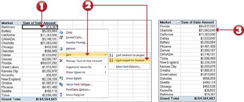
1. Right-click any value within the target field.
2.
Select Sort followed by the sort direction. In this case, the data is
sorted on Sales Amount with the largest numbers at the top.
3. Note that the pivot table now sorts the values per your instructions.
Note: Sorting Persists in a Pivot Table
When you
sort data in a standard worksheet, it’s really a one-time event. That is
to say, if you add data to your data table after sorting, you will need
to sort again. In a pivot table, however, the sorting persists. If new
data is introduced to a sorted pivot table, the new value is
automatically sorted and based on the sort rules you implement. There is
no need to reapply the sort. |