It can be frustrating to enter a formula and
have it either return an incorrect value or an error. An important part
of solving the problem is to understand what the error is trying to
tell you. After you have an idea of the problem you’re looking for, you
can use several tools to look deeper into the error.
Error Messages
After entering a formula, you may run into one of the following errors:
#DIV/0!— Occurs when a number is divided by zero.
#N/A—
Occurs when a value isn’t available in the formula; for example, if
you’re doing a lookup function and the lookup value isn’t found.
#NAME?— Occurs when a formula includes unrecognizable text.
#NULL!—
Occurs when an intersection is specified but the areas do not intersect
or if a range operator is incorrect. For example, if you entered
=SUM(A1:A10 B1:B10), you would get the error because the error
separating the ranges is missing. The correct formula would be
=SUM(A1:A10,B1:B10).
#NUM!— Occurs when there is an invalid numeric value in a formula or function.
#REF!—
Occurs when a cell reference isn’t valid; for example, if the cell has
been deleted. This can be difficult to trace because the #REF can occur
within the formula itself—for example, =#REF*A2—and there’s no direct
way to trace back to the original reference.
#VALUE!— Occurs when trying to do math with nonnumeric data; for example, D1+D2 will return the error if D1 is the column header.
######—
This isn’t really an error. It can occur if the column width is not
wide enough for the formula result or if you’re trying to subtract a
later date from an earlier date.
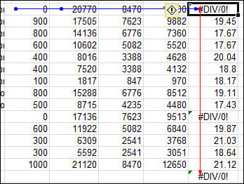
The initial help provided by Excel and Excel Starter
may help trace the problem. When an error cell is selected, an
exclamation icon appears from which you can select Trace Error. If Trace
Error is selected, blue and red lines will appear on the sheet, as
shown in Figure 1.
A red arrow will connect to the first cell causing a problem. From that
cell, blue lines will appear, pointing out the cells used in that
cell’s formula. In Figure 1, the culprits are the 0 quantities being used in the Price Per calculation.
Trace Precedents and Dependents
When you select a cell containing a formula and press
F2, Excel highlights any cells on the sheet that are used by the
formula, but it doesn’t highlight the cells on other sheets. To do that
and more, use the trace precedent and trace dependent auditing arrows.
Use the formula auditing arrows found on the Formulas
tab in the Formula Auditing group if you have a cell you want to trace,
whether it’s to locate other cells used in that cell’s formula or what
cells reference the selected cell. Just select the cell in question and
click a trace button.
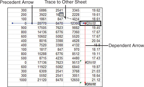
There are two types of auditing arrows:
Trace Precedents— If the selected cell contains a formula, arrows will point to the cells used by the formula.
Trace Dependents— If the selected cell is used in a formula in another cell, arrows will point to the cell containing that formula.
When you click one of the trace buttons, arrows
appear, linking the cell to other cells that are directly connected to
it, as shown in Figure 2.
Click the trace button again and you will get the next level of cell
connections. You can continue to click the button and Excel will
continue adding tracing arrows to the sheet.
If the connecting cell is on another sheet, Excel will display a dashed arrow pointing to a sheet icon, as shown in Figure 5.14.
If you double-click the line, a Go To dialog will appear, listing every
cell containing a link to the selected cell. You can then double-click
one of the listed items and be brought directly to the linked cell.
To clear all the arrows, select Formulas, Formula
Auditing, Remove Arrows. There is no way to go back just one level or
remove one type of arrow.
Watch Window
The
Watch Window found in the Formula Auditing group of the Formulas tab
allows you to watch a cell update as you make changes that will affect
it. This can be useful when you have formulas that span multiple sheets
and you need to watch a cell on one sheet while you make changes to
another.
|
Double-click a cell in the Watch Window to jump to that cell.
|
Watching a Formula Update on Another Sheet
To watch a formula update on another sheet, follow these steps:
1. | Select Formulas, Formula Auditing, Watch Window. The Watch Window dialog appears.
|
2. | Click Add Watch to bring up the Add Watch dialog.
|
3. | Select the cell you want to watch update and click Add.
|
4. | Repeat steps 2 and 3 for any additional cells that you want to monitor.
|
5. | Leave the Watch Window open and make changes to cells that will affect the watched cells.
|
6. | Whether
directly linked or not, if the watched cells are in any way affected by
the changes you make, the Watch Window will update to reflect the new
value of the cell.
|
Evaluating Formulas
If you want to watch how Excel calculates each part of a formula, you can use Formulas, Formula Auditing, Evaluate Formula.
The Evaluate Formula window has three buttons you can
use to investigate a formula. The buttons will work only on the
underlined portion of the formula:
Evaluate— Replaces the underlined portion of the formula with the value.
Step In—
Displays the actual contents of a cell if the underlined portion is a
cell address. This may be a value or a formula. If it’s a formula, you
have the option to continue stepping in until it is resolved.
Step Out— Returns to the previous level of evaluation.
You can continue to evaluate a formula until it is completely resolved.
Using Evaluate to Watch a Formula Calculate
To see how Excel is calculating a formula, follow these steps:
1. | Select the cell with the formula to evaluate.
|
2. | Select Formulas, Formula Auditing, Evaluate Formula.
|
3. | The formula appears in the evaluation window with some part of it underlined.
|
4. | Click the Step In button if it is activated. If it isn’t, skip to step 8.
|
5. | A new section appears in the window, showing the result of the underlined portion.
|
6. | Repeat steps 4 and 5 if the Step In button is still active.
|
7. | When
the Step In button is no longer active, click the Step Out button to
return to the previous level. Each click of the button returns you to
the previous level.
|
8. | Click
the Evaluate button and Excel will evaluate the underlined portion,
replacing it in the formula with the returned or calculated value.
|
9. | Continue to click Evaluate or Step In to watch the formula calculate.
|
10. | Excel
is done with the evaluation when only the calculated value appears in
the Evaluation field. You can either click Restart to go through the
steps again, or click Close to return to Excel.
|
Evaluating with F9
With the Evaluate Window, you have to go in the order
that Excel calculates the formula. If you want to jump directly to a
portion of the formula, you can highlight that portion and press F9 to
evaluate to its value.
You should keep two things in mind when using F9 to evaluate a formula:
When highlighting the portion to evaluate, you must be careful to select the entire portion, including any relevant parentheses.
You must press Esc to leave the cell. If you don’t, Excel will replace your formula with the value you just evaluated to.