Changing the Pivot Table Layout
Excel
2010 gives you a choice of three layouts for your pivot tables. The
three layouts are the Compact Form, Outline Form, and Tabular Form.
Although no layout stands out as being better than the others, the most
popular layout is, by far, the Tabular Form. This is mainly because the
tabular layout was the one that existed in previous versions of Excel,
so most people who have seen pivot tables in the past are used to that
layout.

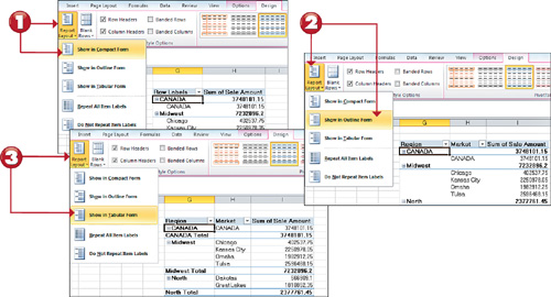
1. Show your pivot table in the Compact layout. Go to the Design tab, click on the Report Layout drop-down and select Show in Compact Form.
2. Show your pivot table in Outline layout. Go to the Design tab, click on the Report Layout drop-down and select Show in Outline Form.
3. Show your pivot table in Tabular layout. Go to the Design tab, click on the Report Layout drop-down and select Show in Tabular Form.
Customizing Field Names
Notice
that every field in your pivot table has a name. The fields in the row,
column, and filter areas inherit their names from the data labels in
your source table. The fields in the Values area are given a name, such
as Sum of Sales Amount. There will often be times when you might prefer
another name for your fields. For instance, you may want your Value
field called Total Sales instead of Sum of Sales Amount.

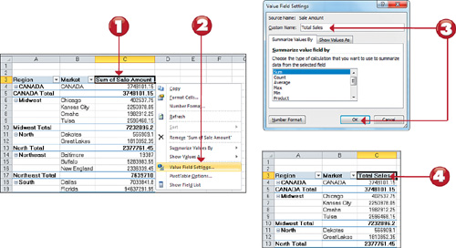
1. Right-click the field Sum of Sales Amount.
2. Select Value Field Settings.
3. Enter the new name in the Custom Name input box and click OK to confirm.
4. Note that the name of your pivot field changed.
Note: Pivot Field Naming Restriction
You
cannot rename a pivot field to the same name used in your source table.
To get around this, you can name the field and add a space to the end of
the name. For example, Excel considers Sales Amount (followed by a
space) to be different from Sales Amount. This way you can use the name
you want, and no one will notice it’s any different. |
Applying Numeric Formats to Data Fields
Numbers
in pivot tables can be formatted to fit your needs (that is, formatted
as currency, percentage, or number). You can easily control the numeric
formatting of a field using the Value Field Settings dialog box.

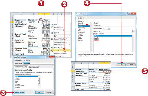
1.
Right-click any value within the target field. For example, if you want
to change the format of the values in the Sales Amount field,
right-click any value under that field.
2. Select Value Field Settings.
3. The Value Field Settings dialog box appears. Click the Number Format button.
4.
The Format Cells dialog box activates. Apply the number format you
desire, just as you normally would on your spreadsheet. Click OK to apply the changes.
5.
After you set the formatting for a field, the applied formatting will
persist even if you refresh or rearrange your pivot table.
Tip: Getting to Field Settings from the Ribbon
You can also get to the Value Field Settings dialog box via the Ribbon. Click the Field Settings command under the Options tab. |