1. Table References in Formulas
Names are automatically created when you define a
table. A name for each column and the entire table are created. You can
use these names to simplify references to the data in formulas.
To find the name of the table, select a cell
in the table and go to Table Tools, Design, Properties. The name of the
table will appear in the Table Name field. You can use this name in
formulas to reference the entire table. The names for the columns are
based on the column headers.
In addition to the table and column specifiers, Excel
provides five more. To access these specifiers, you must first type the
table name.
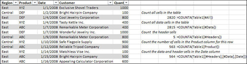
#All— Returns all the contents of the table or specified column.
#Data— Returns the data cells of the table or specified column.
@ (This Row)— Returns the current row.
#Headers— Returns all the column headers or that of a specified column.
#Totals— Returns the total rows or that of a specified column.
Writing Formulas That Refer to Tables
The following are rules for writing formulas that refer to tables:
The reference to the table must start with
the table name. If the formula is within the table itself, you can omit
the table name.
Specifiers, such as a column name or the total row, must be enclosed in square brackets, like this: TableName[Specifier]
If
using multiple specifiers, each specifier must be surrounded by square
brackets and separated by commas. The entire group of specifiers used
must be surrounded by square brackets, like this:
TableName[[Specifier1],[Specifier2]]
If no specifiers are used, the table name refers to the data rows in the table. This does not include the headers or total rows.
The @ (This Row) specifier must be used with another specifier, like this: TableName[[@Specifier]]
Figure 1 shows examples of using specifiers.
2. Using Array Formulas
|
Array formulas cannot be created in the Web App, but they will still calculate in an uploaded file.
|
An array holds multiple values individually in a single cell. An array formula allows you to do calculations with those individual values.
It’s hard to imagine, but three keys on your
keyboard can turn the right formula into a SUPER formula. Three keys
can take 10,000 individual formulas and reduce them
to a single formula. These three keys are Ctrl+Shift+Enter. Enter the
right type of formula in a cell, but instead of just pressing Enter,
press Ctrl+Shift+Enter and the formula becomes an array formula, also
known as a CSE formula.
For example, with an array formula you can do the following:
Multiply corresponding cells together and return the sum or average, as shown in Example 2.
Return a list of the top nth items in a list, while calculating the value by which you are judging their rank, as shown in Example 3.
Sum (or average) only numbers that meet a certain condition, such as falling between a specified range.
Count the number or records that match multiple criteria.
Example 1
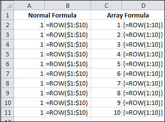
Look at Figure 2.
The ROW function returns the row number of what is in the parentheses.
In columns A and B, you see the result of a normally entered ROW
function looking at rows 1:10—1’s all the way down because the formula
can only return the first value it holds. In columns C and D, you see
the same formula, but entered as an array formula. This time, you can
see each value held in the function—the numbers 1 through 10.
Example 2
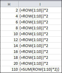
Figure 3
goes to the next step, multiplying each value in the array by 2 as
shown in columns H and I. In cell H10, you include the SUM array
formula, which not only multiplies each value in array by 2, but adds
the results. Imagine if you had a sheet with 10,000 quantities and
prices. Instead of multiplying each row into a new column and then
summing that column, you just have one cell that does the entire
calculation. And because you have fewer formulas, the workbook is
smaller.
Example 3
An array formula can also return multiple values. These values are placed within the range selected before entering the formula.
For example, if you wanted to return the region, product, and date of the top three revenue generators for the data in Figure 4, you would use a formula like this:
=INDEX(A1:A46 & "-" & B1:B46 & " on " &
TEXT(C1:C46,"mm/dd/yy"),MATCH(LARGE(D2:D46*E2:E46,{1;2;3}),(D1:D46*E1:E46)
,0))
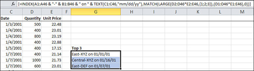
1. | Look for the three largest revenues at the same time they’re being calculated, like this:
LARGE(D2:D46*E2:E46,{1;2;3})
LARGE
is a function that returns the nth largest value in a range, which we
are creating by multiplying corresponding values in columns D and E
(D2*E2, D2*E3 and so forth). In this case, we are looking top three
items and place 1;2;3 in curly brackets. By placing the numbers manually
in curly brackets separated by semi-colons (;), we’re identifying them
as an array.
|
2. | Now that we have the top three values, we have to locate them within the range, like this:
MATCH(LARGE(D2:D46*E2:E46,{1;2;3}),(D1:D46*E1:E46),0)
MATCH returns the row numbers of the calculated revenues by matching
their location within an array of the calculated revenues. The 0 tells
the function we need an exact match to the values.
|
3. | The
formula now holds the rows that the three largest values are found in.
The INDEX function is then used to look up and return the desired
details from those rows.
|
4. | After
you select three cells, type the entire formula and enter it by
pressing Ctrl+Shift+Enter, Excel copies the formula down to each of the
three cells. The first cell returns the first answer in the calculated
array, the second cell returns the second value in the calculated array,
and the third cell returns the third value.
|
When an array formula is holding more than one
calculated value, you must select a range at least the size of the most
values it is returning before entering it and pressing the CSE
combination. If the range selected is too small, only some of the values
will be returned. If the range selected is too large, an error will
appear in the extra cells. Because you have the same formula in multiple
cells, the workbook is smaller; Excel has to track only a single
formula.
Editing Array Formulas
Following are a few rules to use when editing multicell array formulas:
- You cannot edit just one cell of an array formula. A change made to one cell affects them all.
- You can increase the size of the range, but not decrease it. To decrease it, you must delete the formula and reenter it.
- You cannot move just a part of the range, but you can move the entire range.
- The range must be continuous—you cannot insert blank cells within it.
Deleting Array Formulas
You cannot delete just one cell of an array formula.
The entire range containing the array formula must be selected before
you can delete it. The message You Cannot Change Part of an Array will
appear if you try to delete just a portion of the range containing the
formula. You can use Go to Special, Current Array to select the entire
array.
If you need to resize an array to be smaller, you will have to delete and reenter it.
Deleting an Array Formula
Follow these steps to select an entire array formula and delete it:
1. | Select a cell in the array formula.
|
2. | Press Ctrl+G to bring up the Go To dialog.
|
3. | Click the Special button in the lower-left corner of the dialog.
|
4. | Select Current Array and click OK.
|
5. | Press Delete on the keyboard to delete the entire array formula range. |